
| 일 | 월 | 화 | 수 | 목 | 금 | 토 |
|---|---|---|---|---|---|---|
| 1 | 2 | 3 | ||||
| 4 | 5 | 6 | 7 | 8 | 9 | 10 |
| 11 | 12 | 13 | 14 | 15 | 16 | 17 |
| 18 | 19 | 20 | 21 | 22 | 23 | 24 |
| 25 | 26 | 27 | 28 | 29 | 30 | 31 |
- learning_rate
- 모델평가
- plot_model
- Pooling Layer
- 뉴스웨일
- 데이터
- 인공지능
- 머신러닝
- Convolution Neural Network
- 크롤링
- bias
- pandas
- Neural Network
- OneHotEncoding
- AWS 입문자를 위한 강의
- fashion mnist
- MaxPooling2D
- 데이터크롤링
- 딥러닝
- AI
- CNN
- CIFAR-10
- 데이터처리
- 데이터분석
- explained AI
- kt에이블스쿨
- NewsWhale
- CNN 실습
- CRISP-DM
- 키워드 기반 뉴스 조회
- Today
- Total
jjinyeok 성장일지
딥러닝 #1 - 딥러닝 개요 Tensorflow & Keras 2022/09/13~2022/09/16 본문
딥러닝 #1 - 딥러닝 개요 Tensorflow & Keras 2022/09/13~2022/09/16
jjinyeok 2022. 9. 13. 17:50이전 과정 AI 모델 해석 및 평가 과정에서 정말 배운것이 많고 인사이트를 보는 능력을 키울 수 있었지만 자소서 쓰는 시간이 오래 걸려 AI 모델 해석 및 평가 강의를 정리하지 못했다. 그러나 딥러닝 강의 이후 시각 지능 딥러닝과 언어 지능 딥러닝을 배우기 때문에 딥러닝을 먼저 정리해야 할 것 같다. 딥러닝을 정리하고 자소서 시즌이 끝나 시간이 조금 날 때 AI 모델 해석 및 평가 강의를 정리하겠다.
1. Linear Regression을 통한 딥러닝
Linear Regression은 Regression문제를 해결하기 위한 모델로 결과적으로 y = w1 * x1 + w2 * x2 + w3 * x3 + w0와 같은 수식이 만들어진다. 이를 뉴럴 네트워크 구조로 만든다면 다음과 같다.

이때 x1, x2, x3는 Input Layer, y는 Output Layer이다. w1, w2, w3로 Input Layer와 Output Layer가 전부 연결되어 있다. 이런 상황을 Densly하다고 한다.
2. Keras로 Linear Regression 구현하기
TensorFlow와 Keras의 코딩 스타일로 Sequential 스타일과 Functional 스타일이 있다. Sequential 스타일이 간편하고 쉽지만 Functional 스타일은 Layer의 커스텀이 가능하다는 장점이 있기 때문에 두 방법 모두 알아두어야 한다.
첫번째로 Sequential 스타일의 코드에서 모델링은 Layer들을 쌓는 방법으로 진행된다. 먼저 keras.models의 Sequentail() 클래스를 통해 모델을 만들어준다. 이후 모델의 add() 함수에 keras.layer의 Layer들을 입력하여 모델에 Layer들을 쌓을 수 있다. 보스턴 집 값 데이터를 통해 Linear Regression을 구현하는 경우 keras.layer의 Input()을 사용해 Input Layer를 만들 수 있다. Input Layer를 만들 때는 내부 parameter로 shape에 feature의 개수를 입력해야 한다. keras.layer의 Dense()를 사용해 이전 Layer의 노드들과 전부 연결된 Layer를 만들 수 있다. 내부 값으로 Dense로 만들어진 Layer 내부의 노드 개수를 입력해 Layer를 만든다. 과정은 다음과 같다.
'Data: 보스턴 집 값 데이터'
print(x_train.shape, x_val.shape, y_train.shape, y_val.shape)
# (455, 13) (51, 13) (455,) (51,)

'1-1. Sequentail style 모델 생성'
model = keras.models.Sequential()
'1-2. 모델을 차곡차곡 쌓기'
model.add(keras.layers.Input(shape=(13, ))) # feature가 13개인 Input Layer 생성
model.add(keras.layers.Dense(1)) # Layer끼리 모든 노드가 Densly하게 연결
'1-3. 모델 컴파일하기'
model.compile(loss='mse', # 어떤 loss 값을 통해 gradient descent를 진행할지 입력
              optimizer='adam') # gradient descent 과정을 어떻게 진행할지 입력

'2. 모델 학습하기'
model.fit(x_train, y_train,
          epochs=1000, # 학습 데이터를 총 몇번이나 학습시킬지
          verbose=1) # verbose=1 : 학습되는 과정을 보여줌

'3. 모델 평가하기'
pred = model.predict(x_val)
rmse = mean_squared_error(y_val, pred, squared=True)
print(f'rmse: {rmse}')
# rmse: 17.301074161419464
두번째로 Functional 스타일의 코드에서 모델링은 먼저 이전 Layer와 사슬로 연결하듯 엮으며 Layer를 선언하고 이후 Layer들을 사용해 모델을 만든다는 점에서 차이가 있다. 과정은 다음과 같다.
'Data: 보스턴 집 값 데이터'
print(x_train.shape, x_val.shape, y_train.shape, y_val.shape)
# (455, 13) (51, 13) (455,) (51,)

'1-1. Layer 생성'
input_layer = keras.layers.Input(shape=(13, ))
output_layer = keras.layers.Dense(1)(input_layer) # 이전 Layer와 사슬로 연결하듯 연결하기
'1-2. Layer를 parameter로 사용해 모델 생성'
model = keras.models.Model(inputs=input_layer, outputs=output_layer) #inputs와 outputs에 Layer 입력
'1-3. 모델 컴파일하기'
model.compile(loss='mse', # 어떤 loss 값을 통해 gradient descent를 진행할지 입력
              optimizer='adam') # gradient descent 과정을 어떻게 진행할지 입력

'2. 모델 학습하기'
model.fit(x_train, y_train,
          epochs=1000, # 학습 데이터를 총 몇번이나 학습시킬지
          verbose=1) # verbose=1 : 학습되는 과정을 보여줌

'3. 모델 평가하기'
pred = model.predict(x_val)
rmse = mean_squared_error(y_val, pred, squared=True)
print(f'rmse: {rmse}')
# rmse: 40.74972471486908
3. Logistic Regression을 통한 딥러닝
Logistic Regression은 Linear Regression과 다르게 이진 Classification 문제를 해결하기 위한 모델이다. y = w1 * x1 + w2 * x2 + w3 * x3 + w0와 같은 수식에 Sigmoid 함수(Logistic 함수)를 적용해 0과 1 사이의 값으로 만들어 분류 확률을 구하는 모델이다. 확률이 trashold를 기준으로 이상이면 class에 해당, 이하면 class에 해당하지 않게 된다. 따라서 앞선 Linear Regression의 Output Layer 값을 0과 1 사이로 조절하는 추가 조작이 필요하다. 이를 뉴럴 네트워크로 나타내면 다음과 같다.

Logistic Regression은 Linear Regression에서 Output Layer에 sigmoid 함수를 추가해 조작한 모델이다.
4. Keras로 Logistic Regression 구현하기
Logistic Regression의 구현은 Linear Regression의 구현과 크게 3가지가 다르다. 첫째 Logistic Regression은 Output Layer에서 Activation 함수로 Sigmoid 함수를 써야한다. 둘째 Classification 문제기 때문에 Loss를 구할 때 Cross Entropy를 사용하는데 Logistic Regression은 Binary Classification 문제를 해결하는 모델이므로 Binary Cross Entropy를 사용해 Loss를 구해야 한다. 셋째 이때 Binary Cross Entropy는 직관적이지 않기 때문에 추가적으로 Accuracy를 보여준다. 이에 따라 Sequential 스타일의 코드에서 Logistic Regression 모델의 구현은 다음과 같다.
'Data: 유방암 발병 여부 데이터'
print(x_train.shape, x_val.shape, y_train.shape, y_val.shape)
# (512, 30) (57, 30) (512,) (57,)

'1-1. Sequentail style 모델 생성'
model = keras.models.Sequential()
'1-2. 모델을 차곡차곡 쌓기'
model.add(keras.layers.Input(shape=(30, ))) # feature가 30개인 Input Layer 생성
model.add(keras.layers.Dense(1, activation='sigmoid')) # Sigmoid 함수를 activation 함수로 사용해 값을 0과 1 사이의 확률값으로 줄임
'1-3. 모델 컴파일하기'
model.compile(loss='binary_crossentropy', # loss 값으로 Cross Entropy를 이용 현재 이진 분류기 때문에 binary_crossentropy 사용
              optimizer='adam',
              metrics=['accuracy']) # binary_crossentropy는 직관적이지 않기 때문에 정확도(accuracy)도 나타냄

'2. 모델 학습하기'
model.fit(x_train, y_train,
          epochs=1000, # 학습 데이터를 총 몇번이나 학습시킬지
          verbose=1) # verbose=1 : 학습되는 과정을 보여줌

'3. 모델 평가하기'
pred = model.predict(x_val)
pred = np.where(pred >= 0.5, 1, 0) # 0.5를 threshold로 삼음
print(classification_report(y_val, pred))
#               precision    recall  f1-score   support

#            0       0.90      0.90      0.90        21
#            1       0.94      0.94      0.94        36

#     accuracy                           0.93        57
#    macro avg       0.92      0.92      0.92        57
# weighted avg       0.93      0.93      0.93        57
Functional 스타일의 코드에서 Logistic Regression 모델의 구현은 다음과 같다. Linear Regression 코드와 큰 차이가 없음을 기억하면 좋을 것 같다.
'Data: 유방암 발병 여부 데이터'
print(x_train.shape, x_val.shape, y_train.shape, y_val.shape)
# (512, 30) (57, 30) (512,) (57,)

'1-1. Layer 생성'
input_layer = keras.layers.Input(shape=(30,))
output_layer = keras.layers.Dense(1, activation='sigmoid')(input_layer) # 이전 Layer와 사슬로 연결하듯 연결하기
'1-2. Layer를 parameter로 사용해 모델 생성'
model = keras.models.Model(inputs=input_layer, outputs=output_layer) #inputs와 outputs에 Layer 입력
'1-3. 모델 컴파일하기'
model.compile(loss='binary_crossentropy',
              optimizer='adam',
              metrics=['accuracy'])

'2. 모델 학습하기'
model.fit(x_train, y_train,
          epochs=1000, # 학습 데이터를 총 몇번이나 학습시킬지
          verbose=1) # verbose=1 : 학습되는 과정을 보여줌

'3. 모델 평가하기'
pred = model.predict(x_val)
pred = np.where(pred >= 0.5, 1, 0) # 0.5를 threshold로 삼음
print(classification_report(y_val, pred))
#               precision    recall  f1-score   support

#            0       1.00      0.94      0.97        17
#            1       0.98      1.00      0.99        40

#     accuracy                           0.98        57
#    macro avg       0.99      0.97      0.98        57
# weighted avg       0.98      0.98      0.98        57
5. Multi-Class Classification
앞선 Logistic Regression은 Binary Classification 문제 해결을 위한 모델이다. 3개 이상의 Class에 대해 Classification을 분류하기 위해서는 Logistic Regression이 아닌 다른 Classification 모델이 필요하다. 먼저 3개 이상의 Class에 대해 Classification을 하기 위해서는 각 Class에 별로 Logisitic Regression 해야 함을 의미한다. 하나의 Class(One)과 나머지 Class들(Rest)을 분리하는 것이다. (One vs. Rest 또는 One vs. The others) 따라서 Target의 형태를 Class 수만큼으로 바꿔야 한다. 이것을 One-Hot Encoding이라 한다. 이때 keras.utils의 to_categorical() 함수를 사용한다. 내부에 Target y와 Class 수 n을 입력해 Target의 형태를 바꿀 수 있다.
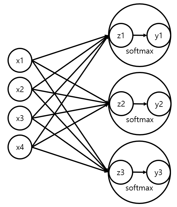
Multi-Class Classification이란 여러 Class 중 하나의 Class를 선택하는 것이다. 따라서 Activation 함수로 Softmax를 사용해 각 Class일 확률을 구하는 방법을 사용한다. Softmax를 사용하면 결과값으로 각 Class일 확률이 Numpy의 Array 형식으로 출력된다. 이때 Numpy Array의 argmax() 메서드를 이용하여 가장 높은 값의 Class를 구해 모델을 평가할 수 있다. 또한 Classification 문제기 때문에 Loss를 구할 때 Cross Entropy를 사용하는데 Categorical Cross Entropy를 사용한다. 이를 뉴럴 네트워크로 나타내면 다음과 같다.
Sequential 스타일의 코드에서 Multi-Class Classification 모델의 구현은 다음과 같다.
'Data: 3가지 붓꽃 종 (setosa, versicolor, virginica) 분류 데이터'

'One Hot encoding'
y_train = to_categorical(y_train, 3)
y_val = to_categorical(y_val, 3)
print(x_train.shape, x_val.shape, y_train.shape, y_val.shape)
# (135, 4) (15, 4) (135, 3) (15, 3)

'1-1. Sequentail style 모델 생성'
model = keras.models.Sequential()
'1-2. 모델을 차곡차곡 쌓기'
model.add(keras.layers.Input(shape=(4, )))
model.add(keras.layers.Dense(3, activation='softmax'))
'1-3. 모델 컴파일하기'
model.compile(loss='categorical_crossentropy', # Multi-Class Classification의 loss
              optimizer='adam',
              metrics=['accuracy'])

'2. 모델 학습하기'
model.fit(x_train, y_train, epochs=1000, verbose=1)

'3. 모델 평가하기'
pred = model.predict(x_val)
pred = pred.argmax(axis=1) # argmax() 메서드를 통해 예측 Class 확인
y_val = y_val.argmax(axis=1) # argmax() 메서드를 통해 정답 Class 확인
print(classification_report(y_val, pred))
#               precision    recall  f1-score   support

#            0       1.00      1.00      1.00         3
#            1       1.00      0.89      0.94         9
#            2       0.75      1.00      0.86         3

#     accuracy                           0.93        15
#    macro avg       0.92      0.96      0.93        15
# weighted avg       0.95      0.93      0.94        15
Functional 스타일의 코드에서 Multi-Class Classification 모델의 구현은 다음과 같다.
'Data: 3가지 붓꽃 종 (setosa, versicolor, virginica) 분류 데이터'

'One Hot encoding'
y_train = to_categorical(y_train, 3)
y_val = to_categorical(y_val, 3)
print(x_train.shape, x_val.shape, y_train.shape, y_val.shape)
# (135, 4) (15, 4) (135, 3) (15, 3)

'1-1. Layer 생성'
input_layer = keras.layers.Input(shape=(4, ))
output_layer = keras.layers.Dense(3, activation='softmax')(input_layer)
'1-2. Layer를 parameter로 사용해 모델 생성'
model = keras.models.Model(inputs=input_layer, outputs=output_layer)
'1-3. 모델 컴파일하기'
model.compile(loss='categorical_crossentropy', # Multi-Class Classification의 loss
              optimizer='adam',
              metrics=['accuracy'])

'2. 모델 학습하기'
model.fit(x_train, y_train, epochs=1000, verbose=1)

'3. 모델 평가하기'
pred = model.predict(x_val)
pred = pred.argmax(axis=1) # argmax() 메서드를 통해 예측 Class 확인
y_val = y_val.argmax(axis=1) # argmax() 메서드를 통해 정답 Class 확인
print(classification_report(y_val, pred))
#               precision    recall  f1-score   support

#            0       1.00      1.00      1.00         8
#            1       1.00      1.00      1.00         4
#            2       1.00      1.00      1.00         3

#     accuracy                           1.00        15
#    macro avg       1.00      1.00      1.00        15
# weighted avg       1.00      1.00      1.00        15
6. 정리하기
| Linear Regression | Rogistic Regression | Multi-Class Classification | |
| Ouput Layer Activation |
linear (생략 가능) | sigmoid | softmax |
| Loss | mse (mae, mape 가능하지만 mse 많이 씀) | binary_crossentropy | categorical_crossentropy |
오늘 배운 모델은 사실 딥러닝이 아니다. 그저 Tensorflow와 Keras를 통한 머신러닝의 구현이었다. 그러나 Tensorflow와 Keras의 문법을 알게 되었고 이를 통해 앞으로 있을 딥러닝을 배우는 과정은 더 수월할 수 있을 것이다.
'[KT AIVLE School]' 카테고리의 다른 글
| 딥러닝 #3 - 적용하기 2022/09/13~2022/09/16 (0) | 2022.09.16 |
|---|---|
| 딥러닝 #2 - ANN 2022/09/13~2022/09/16 (0) | 2022.09.15 |
| 머신 러닝 #5 - Ensemble 기법 2022/08/22~2022/08/29 (0) | 2022.09.12 |
| 머신 러닝 #4 - 성능 튜닝 2022/08/22~2022/08/29 (0) | 2022.09.11 |
| 머신 러닝 #3 - Decision Tree & SVM 2022/08/22~2022/08/29 (0) | 2022.08.30 |


