
| 일 | 월 | 화 | 수 | 목 | 금 | 토 |
|---|---|---|---|---|---|---|
| 1 | 2 | 3 | 4 | 5 | ||
| 6 | 7 | 8 | 9 | 10 | 11 | 12 |
| 13 | 14 | 15 | 16 | 17 | 18 | 19 |
| 20 | 21 | 22 | 23 | 24 | 25 | 26 |
| 27 | 28 | 29 | 30 |
- 크롤링
- kt에이블스쿨
- bias
- 데이터처리
- plot_model
- 머신러닝
- learning_rate
- CNN 실습
- MaxPooling2D
- pandas
- 키워드 기반 뉴스 조회
- explained AI
- 뉴스웨일
- AWS 입문자를 위한 강의
- Convolution Neural Network
- CIFAR-10
- 데이터분석
- NewsWhale
- 모델평가
- AI
- 인공지능
- Pooling Layer
- fashion mnist
- OneHotEncoding
- CRISP-DM
- Neural Network
- 딥러닝
- 데이터크롤링
- CNN
- 데이터
- Today
- Total
jjinyeok 성장일지
딥러닝 #3 - 적용하기 2022/09/13~2022/09/16 본문
1. 왜 딥러닝인가?
지금까지 머신러닝을 배웠다. 지금까지 배웠던 머신러닝의 과정에서 Feature를 추출하고 모델에 적용하는 과정에서 사람은 Feature의 선택과 가공을 조절하게 된다. 즉 지금까지 배웠던 과정에서 Feature Engineering은 필수적이다. 그러나 딥러닝을 이용한 모델은 사람이 Feature를 직접 조절하고 선택하지 않는다. 모델이 직접 Feature를 조절하고 선택한다. 사람은 단지 Node의 개수를 통해 Feature의 양과 Layer 개수를 통해 Feature의 수준만 조절한다. 딥러닝을 이용하면 사람이 보지 못했던 Feature를 파악할 수 있다. 따라서 이미지와 자연어와 같은 잘 정제되지 않은 데이터에서 딥러닝 모델을 사용하는 것이 유리하다.
2. Fashion MNIST에서 ANN 적용하기
Fashion MNIST에 ANN을 적용하는 과정은 앞선 MNIST 데이터와 데이터만 다를 뿐 코드는 동일하다. 좀 더 다양한 분야에서 ANN을 적용하는 방법이라고 생각하자. 코드는 다음과 같다.
import tensorflow as tf
from tensorflow import keras
from tensorflow.keras.backend import clear_session
from tensorflow.keras.models import Sequential, Model
from tensorflow.keras.layers import Input, Dense, Flatten
from tensorflow.keras.losses import categorical_crossentropy
from tensorflow.keras.optimizers import Adam
from tensorflow.keras.activations import relu, softmax

(x_train, y_train), (x_test, y_test) = keras.datasets.fashion_mnist.load_data()
print(x_train.shape, x_test.shape, y_train.shape, y_test.shape)
# (60000, 28, 28) (10000, 28, 28) (60000,) (10000,)
# Define the text labels
fashion_mnist_labels = ["T-shirt/top",  # index 0
                        "Trouser",      # index 1
                        "Pullover",     # index 2
                        "Dress",        # index 3
                        "Coat",         # index 4
                        "Sandal",       # index 5
                        "Shirt",        # index 6
                        "Sneaker",      # index 7
                        "Bag",          # index 8
                        "Ankle boot"]   # index 9

'1. 전처리'
# MinMax Scaling
x_train = (x_train - x_train.min()) / (x_train.max() - x_train.min())
x_test = (x_test - x_test.min()) / (x_test.max() - x_test.min())
print(f'max: {x_train.max()} / min: {x_train.min()}')
# max: 1.0 / min: 0.0

# One Hot Encoding
from tensorflow.keras.utils import to_categorical
y_train = to_categorical(y_train)
y_test = to_categorical(y_test)
print(y_train.shape)
# (60000, 10)

'2. 모델링'
clear_session()

model = Sequential()

model.add(Input(shape=(x_train.shape[1], x_train.shape[2])))
model.add(Flatten())
model.add(Dense(256, activation=relu))
model.add(Dense(256, activation=relu))
model.add(Dense(256, activation=relu))
model.add(Dense(10, activation=softmax))

model.compile(loss=categorical_crossentropy,
              optimizer=Adam(),
              metrics=['accuracy']
              )

print(model.summary())
# Model: "sequential"
# _________________________________________________________________
#  Layer (type)                Output Shape              Param #
# =================================================================
#  flatten (Flatten)           (None, 784)               0

#  dense (Dense)               (None, 256)               200960

#  dense_1 (Dense)             (None, 256)               65792

#  dense_2 (Dense)             (None, 256)               65792

#  dense_3 (Dense)             (None, 10)                2570

# =================================================================
# Total params: 335,114
# Trainable params: 335,114
# Non-trainable params: 0
# _________________________________________________________________
# None

'3. 학습'
from tensorflow.keras.callbacks import EarlyStopping
es = EarlyStopping(monitor='val_loss',
                   min_delta=0,
                   patience=5,
                   verbose=1,
                   restore_best_weights = True,
                   )
model.fit(x_train, y_train, epochs=100, verbose=1,
          validation_split=0.2,
          callbacks=[es],
          )

'4. 평가'
from sklearn.metrics import accuracy_score

pred_train = model.predict(x_train)
pred_test = model.predict(x_test)

single_pred_train = pred_train.argmax(axis=1)
single_pred_test = pred_test.argmax(axis=1)

logi_train_accuracy = accuracy_score(y_train.argmax(axis=1), single_pred_train)
logi_test_accuracy = accuracy_score(y_test.argmax(axis=1), single_pred_test)

print('트레이닝 정확도 : {:.2f}%'.format(logi_train_accuracy*100))
print('테스트 정확도 : {:.2f}%'.format(logi_test_accuracy*100))
# 트레이닝 정확도 : 92.92%
# 테스트 정확도 : 89.30%
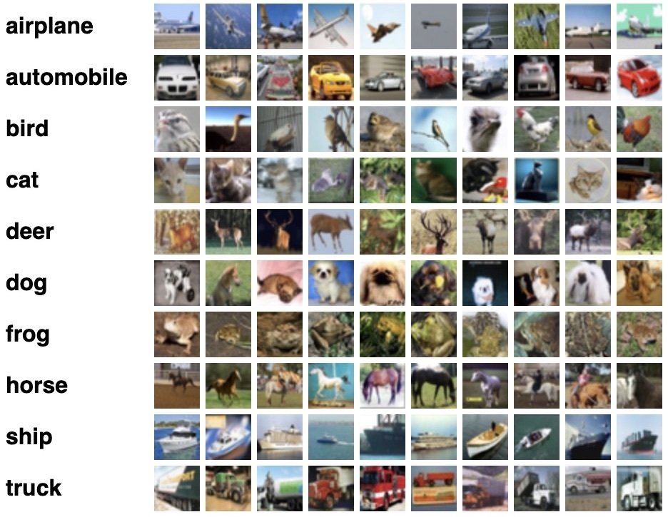
3. CIFAR-10에서 ANN 적용하기
CIFAR-10 데이터 셋은 머신 러닝 및 컴퓨터 비전 알고리즘을 훈련하는 데 일반적으로 사용되는 이미지 모음이다. 이전 MNIST 데이터셋, Fashion MNIST 데이터셋과는 다르게 rgb로 색이 존재하여 Feature 수가 3인 차원이 하나 추가되어 있다. CIFAR-10에서 이전에 사용하던 방식대로 ANN을 적용하였다. 그 과정은 다음과 같다.
import tensorflow as tf
from tensorflow import keras

(train_x, train_y), (test_x, test_y) = keras.datasets.cifar10.load_data()
print(train_x.shape, train_y.shape, test_x.shape, test_y.shape)
# (50000, 32, 32, 3) (50000, 1) (10000, 32, 32, 3) (10000, 1)
# Define the text labels
labels = { 0 : 'Airplane',
          1 : 'Automobile',
          2 : 'Bird',
          3 : 'Cat',
          4 : 'Deer',
          5 : 'Dog',
          6 : 'Frog',
          7 : 'Horse',
          8 : 'Ship',
          9 : 'Truck' }

'1. 전처리'
from tensorflow.keras.utils import to_categorical
x_train = (x_train - x_train.min()) / (x_train.max() - x_train.min())
y_train = to_categorical(y_train, len(np.unique(y_train)))
y_test = to_categorical(y_test, len(np.unique(y_test)))

'2. 모델링'
keras.backend.clear_session()

model = keras.models.Sequential()
model.add(keras.layers.Input(shape=(32, 32, 3)))
model.add(keras.layers.Flatten())
model.add(keras.layers.Dense(512, activation=keras.activations.relu))
model.add(keras.layers.Dense(512, activation=keras.activations.relu))
model.add(keras.layers.Dense(256, activation=keras.activations.relu))
model.add(keras.layers.Dense(128, activation=keras.activations.relu))
model.add(keras.layers.Dense(10, activation=keras.activations.softmax))
model.compile(loss=keras.losses.categorical_crossentropy,
              optimizer=keras.optimizers.Adam(),
              metrics=['accuracy'],
              )

print(model.summary())
# Model: "sequential"
# _________________________________________________________________
#  Layer (type)                Output Shape              Param #
# =================================================================
#  flatten (Flatten)           (None, 3072)              0

#  dense (Dense)               (None, 512)               1573376

#  dense_1 (Dense)             (None, 512)               262656

#  dense_2 (Dense)             (None, 256)               131328

#  dense_3 (Dense)             (None, 128)               32896

#  dense_4 (Dense)             (None, 10)                1290

# =================================================================
# Total params: 2,001,546
# Trainable params: 2,001,546
# Non-trainable params: 0
# _________________________________________________________________
# None

'3. 학습'
from tensorflow.keras.callbacks import EarlyStopping
es = EarlyStopping(monitor='val_loss',
                   min_delta=0,
                   patience=5,
                   verbose=1,
                   restore_best_weights = True,
                   )
model.fit(x_train, y_train, epochs=100, verbose=1,
          validation_split=0.2,
          callbacks=[es],
          )

'4. 평가'
from sklearn.metrics import accuracy_score

pred_train = model.predict(x_train)
pred_test = model.predict(x_test)

single_pred_train = pred_train.argmax(axis=1)
single_pred_test = pred_test.argmax(axis=1)

logi_train_accuracy = accuracy_score(y_train.argmax(axis=1), single_pred_train)
logi_test_accuracy = accuracy_score(y_test.argmax(axis=1), single_pred_test)

print('트레이닝 정확도 : {:.2f}%'.format(logi_train_accuracy*100))
print('테스트 정확도 : {:.2f}%'.format(logi_test_accuracy*100))
# 트레이닝 정확도 : 54.83%
# 테스트 정확도 : 40.25%
그러나 이전 MNIST나 Fashion MNIST에 비해 성능은 낮은 모습을 보인다. 비록 10개 중 하나를 선택하는 과정에서 정확도가 40%라면 찍는 확률인 10%보다 높다. 그러나 이런 모델을 사용할 수는 없다. 이것은 Flatten을 통해 3차원 데이터를 전부 1개의 차원으로 만들어서 생긴 문제이다. 따라서 이런 문제를 해결하기 위해 Convolutional Neural Network (CNN)을 사용한다. 다음주 시각지능 인공지능에서 CNN을 1주일 간 배운다고 하니 기대가 된다.
4. Connection 조절하기
Fully Connected된 Multi Layer Perceptron에서 각 Node(Feature)가 어떤 역할을 하는지 알기가 어렵다. 또한 사람의 의도를 모델링에 직접적으로 반영하는 것 또한 어렵다. 그러나 우리는 모델링을 진행하며 Node의 연결을 직접 관여해 제어할 수 있다.
5. Iris 데이터에서 Connection 조절하기
Iris는 붓꽃 종 데이터이다. 이때 Input Feature로 잎의 높이, 너비와 꽃받침의 높이, 너비가 주어진다. 잎의 높이와 꽃받침의 높이를 묶고 잎의 너비와 꽃받침의 너비를 엮어 Connection을 조절한 모델을 만들 수 있다. 모델은 다음과 같이 구성될 것이다.
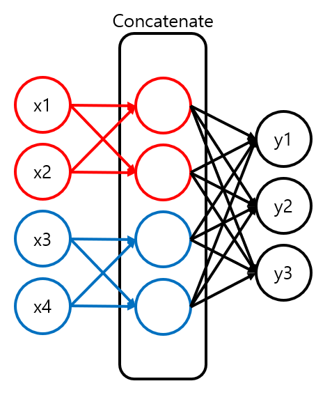
먼저 묶을 Input Feature끼리 분리한다. 분리된 Feature끼리 묶을 수 있도록 Node들을 생성한다. 이것을 Concatenate해 하나의 Layer로 만들고 이것을 통해 Target 구하는 모델을 만들 수 있다. 전체 과정을 코드로 구현하면 다음과 같다.
'1. 전처리'
# Train Set, Test Set 구분
from sklearn.model_selection import train_test_split

x_train, x_test, y_train, y_test = train_test_split(df_x, y, test_size=0.2)
print(x_train.shape, x_test.shape, y_train.shape, y_test.shape)
# (120, 4) (30, 4) (120,) (30,)

# x 분리: length 끼리, width 끼리
x_train_length = x_train.loc[:, ['sepal length (cm)', 'petal length (cm)'] ]
x_train_width = x_train.loc[:, ['sepal width (cm)', 'petal width (cm)'] ]

x_test_length = x_test.loc[:, ['sepal length (cm)', 'petal length (cm)'] ]
x_test_width = x_test.loc[:, ['sepal width (cm)', 'petal width (cm)'] ]

# One Hot Encoding
from tensorflow.keras.utils import to_categorical

y_train = to_categorical(y_train, 3)
y_test = to_categorical(y_test, 3)

'2. 모델링'
input_layer_length = keras.layers.Input(shape=(2, ), name='input_length')
input_layer_width = keras.layers.Input(shape=(2, ), name='input_width')

hidden_layer_lenght = keras.layers.Dense(2, activation='swish', name='hidden_lenght')(input_layer_length)
hidden_layer_width = keras.layers.Dense(2, activation='swish', name='hidden_width')(input_layer_width)
hidden_layer_concat = keras.layers.Concatenate(name='concatenate')([hidden_layer_lenght, hidden_layer_width])

output_layer = keras.layers.Dense(3, activation='softmax', name='output')(hidden_layer_concat)

model = keras.models.Model(inputs=[input_layer_length, input_layer_width], outputs=output_layer)

model.compile(loss='categorical_crossentropy', optimizer='adam', metrics=['accuracy'])

'3. 학습'
es = EarlyStopping(monitor='val_loss',
                   min_delta=0,
                   patience=5,
                   verbose=1,
                   restore_best_weights=True)

model.fit([x_train_length, x_train_width], y_train, epochs=1000, verbose=1,
          callbacks=[es],
          validation_split=0.1,
          )

'4. 평가'
from sklearn.metrics import classification_report
pred = model.predict([x_test_length, x_test_width])
print(classification_report(y_test.argmax(axis=1), pred.argmax(axis=1)))
#               precision    recall  f1-score   support

#            0       1.00      1.00      1.00        12
#            1       1.00      0.89      0.94         9
#            2       0.90      1.00      0.95         9

#     accuracy                           0.97        30
#    macro avg       0.97      0.96      0.96        30
# weighted avg       0.97      0.97      0.97        30
이때 주의해야 할점은 Functional 스타일의 딥러닝 모델에서만 적용이 가능하다는 것이다. 또한 Concatenate가 아닌 Add와 Subtract을 통해 분리된 Layer들을 묶는 것도 가능하다는 것도 유의하자. 코드를 통해 만든 모델을 tensorflow.keras.utils의 plot_model() 함수를 통해 볼 수 있다. 과정과 결과는 다음과 같다.
# 모델 시각화
from tensorflow.keras.utils import plot_model
plot_model(model, show_shapes=True)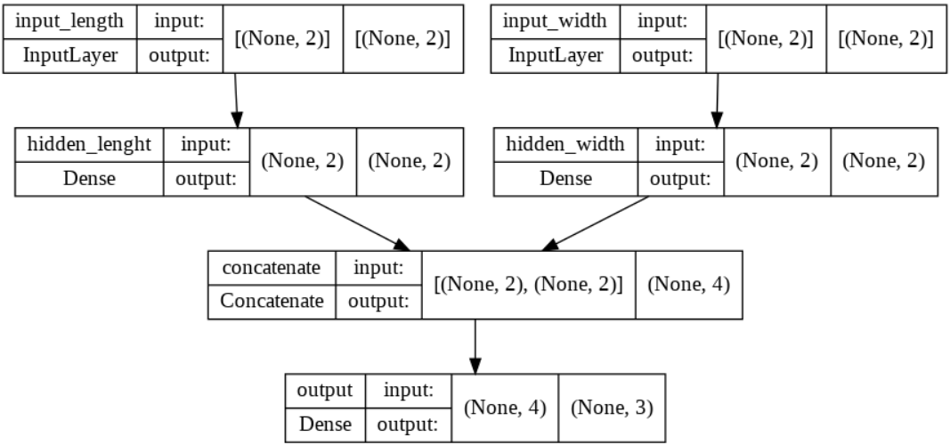
'[KT AIVLE School]' 카테고리의 다른 글
| 시각지능 딥러닝 #2 - CNN 실습 2022/09/19~2022/09/23 (0) | 2022.09.20 |
|---|---|
| 시각지능 딥러닝 #1 - CNN 개요 2022/09/19~2022/09/23 (0) | 2022.09.19 |
| 딥러닝 #2 - ANN 2022/09/13~2022/09/16 (0) | 2022.09.15 |
| 딥러닝 #1 - 딥러닝 개요 Tensorflow & Keras 2022/09/13~2022/09/16 (0) | 2022.09.13 |
| 머신 러닝 #5 - Ensemble 기법 2022/08/22~2022/08/29 (0) | 2022.09.12 |


